Presently, the Transformer architecture constitutes the foundation for nearly all advanced generative artificial intelligence models. However, when attempting to comprehend their internal mechanisms, developers frequently encounter two extremes: either overly simplistic metaphors or the dense academic mathematics from the original 2017 paper, Attention Is All You Need.
In this guide, the Transformer architecture will be analyzed as a rigorous, sequential industrial pipeline. The objective of this study is to trace the exact path of input data from raw text to the prediction of the next token. In order to maintain fidelity with the computational processes of large language models, all data and context examples will be constructed using the phrase “The cat sat on the mat”. The objective is to comprehend the mathematical and logical framework underlying this process while maintaining a focus on the nuances.
Table of Contents
Stage 1. Raw material preparation through tokenization
Neural networks cannot directly process letters or words in their raw form. The first part of our pipeline is the tokenizer. That’s a module that converts a string of characters into an array of numerical identifiers. Today’s transformers typically use algorithms like Byte Pair Encoding (BPE) or WordPiece for tokenization. The algorithm doesn’t just split the text by spaces; it divides it into frequently occurring fragments, roots, suffixes, and punctuation marks. This elegantly solves the problem of unknown words. If a model has never seen a whole word, it’ll just put it together from the familiar pieces it knows.
For our test phrase, the model’s vocabulary looks fixed, with each element assigned its own unique numerical index.
| Original word | Extracted token | Vocabulary ID |
|---|---|---|
| The | “The” | 464 |
| cat | “cat” | 3797 |
| sat | “sat” | 3332 |
| on | “on” | 319 |
| the | “the” | 262 |
| mat | “mat” | 12033 |
Leaving the tokenizer, we receive a one-dimensional array of integers.
Input IDs = [464, 3797, 3332, 319, 262, 12033]It’s important to understand the main limitation of this stage. Right now, the indices 464 and 3797 are just sequence numbers in a table. The model doesn’t yet know that a cat is a living creature or that a mat is an inanimate object. To the network, these are isolated entities with no context.
Stage 2. Digitizing meanings in the embedding space
To turn flat token indices into rich semantic structures, the data is passed to the embedding layer. An embedding is basically a way to represent a word as a mathematical vector of a fixed dimension, denoted as dmodel. In the base Transformer, this is equal to 512, while in modern massive language models, it exceeds ten thousand.
Picture a huge chart with thousands of lines, with each line representing a hidden meaning: whether something is alive, how big it is, how it’s related to an action, and so on. The model builds these properties during a long training process. Each identifier from the tokenizer table is matched with a row in the embedding weight matrix, turning our token into a vector of real numbers.
Ecat = [0.124, -0.581, 0.912, …, 0.043]
In this space, tokens with similar meanings will have close coordinates and minimal cosine distance between their vectors, while words with different meanings will be pushed far apart. We combine the semantic vectors of all the tokens in our phrase to form the input embedding matrix Xemb with dimensions N by dmodel, where N is the length of our context.
| Token | Dimension and vector structure in matrix Xemb |
|---|---|
| The | [ 0.012, -0.341, 0.115, … 512 values … ] |
| cat | [ 0.124, -0.581, 0.912, … 512 values … ] |
| sat | [ -0.201, 0.042, -0.711, … 512 values … ] |
| on | [ 0.512, -0.112, 0.003, … 512 values … ] |
| the | [ 0.012, -0.341, 0.115, … 512 values … ] |
| mat | [ -0.045, 0.891, -0.212, … 512 values … ] |
Stage 3. The geometry of order through positional encoding
The Transformer is a real architectural powerhouse, but it’s also got a bit of a weak spot. It processes all the data it gets at once, which is pretty impressive. It doesn’t have a built-in way to read from left to right, like older recurrent networks did. If you don’t mess with it, saying the cat sat on the mat and the mat sat on the cat will give you the same set of vectors. The architecture doesn’t care about word order.
To help the model understand sentence structure, we add a matrix of positional signals to the embedding matrix. In the original architecture, interpolated trigonometric functions with alternating frequencies are used for this purpose.
PE(pos, 2i) = sin(pos / 100002i/dmodel)
PE(pos, 2i+1) = cos(pos / 100002i/dmodel)
In these equations, the parameter pos is the position index of the token in the sequence from zero to five, and the symbol i is the index of a specific coordinate within the 512-dimensional vector. The output is a standard matrix addition.
X = Xemb + PE
Thanks to the math behind sines and cosines, the final input matrix now has information encoded in it. The model can calculate not only where a specific token stands, but also how far it is from other words in the context window.
Stage 4. The self-attention mechanism as the heart of the algorithm
Now, the data goes into the most important part of the architecture – the Multi-Head Self-Attention layer. The point of this node is to get the tokens to interact with each other and recalculate their semantic vectors based on the context of their whole surroundings. For example, the word “sat” needs to clearly indicate who was sitting and on what.
To implement this process, the algorithm creates three intermediate vectors for each token. They’re called Query, Key, and Value. We can do this by multiplying our base matrix, X, by three trainable weight matrices.
Q = X × WQ, K = X × WK, V = X × WV
In the case of a base dimension of 512, intermediate vector matrices are typically compressed, for instance, down to a dimension of 64 elements for each of the parallel attention heads.
The attention weight matrix is actually calculated in three simple steps. First, the model calculates the dot product of the query and key vectors. It takes the query vector of the first token and multiplies it with all the key vectors of every word in the sentence, including itself. This determines how relevant and connected words are through the matrix multiplication of Q and KT.
Then, in the second step, we scale the raw scores. They’re divided by the square root of the key vectors’ dimension. This is necessary to keep the gradients stable during training, so they don’t get too big before the exponential function. In the third step, the rows of the resulting scaled matrix are passed through a Softmax function. All values are turned into probabilities from zero to one, and the total in each row is always one. That’s the final formula for the attention layer.
Attention(Q, K, V) = Softmax((Q × KT) / √dk) × V
If we look at a specific example of the distribution of these weights for the cat token, after the Softmax operation, the most attention will be directed to the cat token itself (about 45%) and to its associated action sat (about 35%), while only tiny fractions will remain for functional words like the or the spatial mat.
Then, to finish up, the distribution weights are multiplied by the Value vector matrix. Now, the cat token’s vector at the output is enriched with the context of the entire sentence. In real models, this process is run in parallel across multiple threads so that each attention head can track its own types of relationships: one tracks grammatical ties, another spatial ones, and a third temporal dependencies.
Stage 5. Transformation and stabilization through feed-forward networks
After getting the context through the attention mechanisms, the vectors of all tokens go through a normalization block and are sent into a classic Feed-Forward Network. It’s applied to each position the same way, totally independently. The network has two sequential linear transformations with a ReLU or GELU activation function in between.
FFN(Z) = max(0, Z × W1 + b1) × W2 + b2
At this stage, the features are processed in a deep nonlinear way. The main static knowledge base of the neural network is stored in these hidden matrices. The network gathered this knowledge over months of training on terabytes of text.
Residual connections and normalization layers are essential for the stability of the entire pipeline. The input signal of each major block is added to its output signal using the X + Sublayer(X) scheme. This allows the information signal and gradients to pass smoothly through dozens of transformer layers without fading or distorting.
Stage 6. The output gateway and final generation
A modern Transformer is made up of a bunch of these blocks, and the number of blocks can vary from twelve to over a hundred in the most powerful models. After going through all the layers, the original matrix completely changes the numerical values of its vectors. It does this by absorbing all the logical and contextual relationships of the structure.
All that’s left to do is get the final answer and find out exactly which word should continue the phrase. To do this, the vector of the very last processed token, which corresponds to the mat’s position, is fed into the final output computation node.
First, the vector of the last token is projected through a linear layer onto a final weight matrix. This matrix has the same number of columns as the model’s entire massive vocabulary. The result is a list of raw scores, called logits, where each known word is assigned a specific number. Then, these logits are transformed through a final Softmax function into a strict probability distribution.
| Vocabulary token | Logit | Final probability |
|---|---|---|
| and | 14.2 | 68.5% |
| sleeping | 12.1 | 22.1% |
| purred | 10.3 | 4.8% |
| the | 5.1 | 0.2% |
| spaceship | -4.2 | 0.00001% |
The algorithm picks the most suitable token based on the selected generation strategy. For us, that’s the conjunction “and.” It’s translated back into text right away and sent to the user, and its numerical ID is added to the end of the original set of Input IDs. Then, the whole pipeline is restarted, but this time for a bigger context that includes the newly generated word.
Stage 7. The invisible guardrails and how AI censorship works
We’ve seen how the model predicts the next word based on pure mathematics. But why won’t it generate a recipe for a dangerous chemical or use foul language when prompted? The basic transformer architecture doesn’t have a moral compass. It just calculates probabilities based on the training data it’s been exposed to, which includes a ton of unfiltered internet text. To make the AI safe and polite, engineers have built a strong system of invisible guardrails around our six-stage pipeline.
The first layer of censorship happens right at the start, even before your text reaches the tokenizer. Whenever you send a message, the app quietly adds a hidden block of instructions called the system prompt. It’s got some pretty strict rules about what the model can and can’t talk about. So, even though you might think your input is just a short question, the transformer actually processes a much larger text. It starts with directives to be a helpful and harmless assistant. This hidden context changes the model’s internal attention mechanisms and calculations, guiding it towards using safe language.
The second and most important layer of control is built into the model’s internal memory during a process called Reinforcement Learning from Human Feedback. During this special training process, human testers evaluate the model’s answers, effectively punishing it for generating inappropriate content. This changes the weights inside the Feed-Forward networks forever. When the model processes a potentially harmful request today, the math simply doesn’t give high probabilities to toxic words. The internal scores for dangerous responses are pushed so far into the negative that the final Softmax function basically makes it so they have no chance of being chosen.
The final line of defense operates completely outside our main pipeline. As the transformer generates text word by word at the final stage, a separate and smaller neural network monitors the output stream in real time like a strict security guard. If this secondary classifier detects that the emerging sequence of words is crossing a forbidden line, it immediately stops the generation process. The raw output is intercepted and destroyed, and the user gets a pre-written refusal template instead.
Can AI really think? Why its intelligence could surprise you